Setup
First, load the metapaths package, as well as other
requisite packages.
# load packages
library(metapaths)
library(data.table)
library(magrittr)

# for comparison and visualization
library(igraph)
#>
#> Attaching package: 'igraph'
#> The following objects are masked from 'package:stats':
#>
#>     decompose, spectrum
#> The following object is masked from 'package:base':
#>
#>     union
Print the example dataset.
mtcars_node_list = get_node_list(mtcars_edge_list)
head(mtcars_node_list)
#> Node NodeType
#> 1: Porsche 914-2 Five
#> 2: Lotus Europa Five
#> 3: Merc 450SLC Three
#> 4: Merc 280 Four
#> 5: Datsun 710 Four
#> 6: Honda Civic Four
head(mtcars_edge_list)
#> Origin Destination OriginType DestinationType
#> 1: Porsche 914-2 Merc 230 Five Four
#> 2: Lotus Europa Fiat 128 Five Four
#> 3: Merc 450SLC Valiant Three Three
#> 4: Merc 280 Duster 360 Four Three
#> 5: Datsun 710 Toyota Corolla Four Four
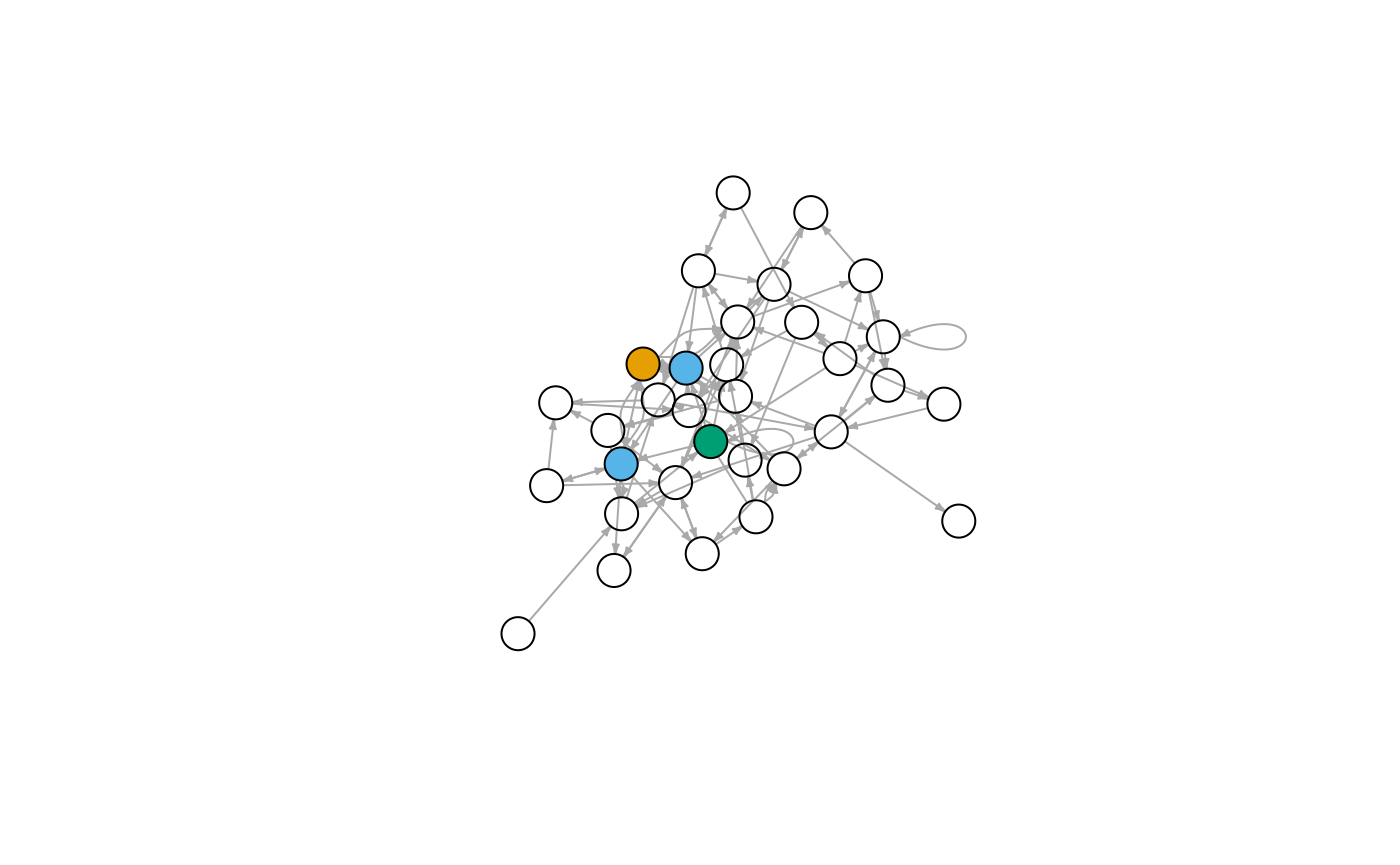
#> 6: Honda Civic Volvo 142E Four FourVisualize the network as a graph.
mtcars_graph = graph.data.frame(mtcars_edge_list, vertices = mtcars_node_list, directed = T)
mtcars_col = factor(V(mtcars_graph)$NodeType)
plot(mtcars_graph, vertex.size = 15, vertex.label = NA, edge.arrow.size = .25, vertex.color = mtcars_col)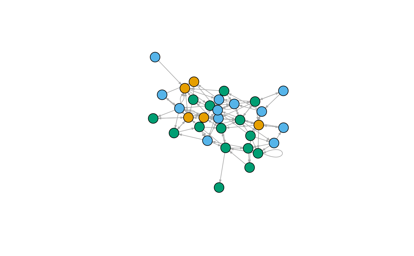
Get all node types.
mtcars_types = node_types(mtcars_edge_list, verbose = T)
#> Node Types:
#> - Five
#> - Three
#> - Four
Retrieve a list of unique nodes.
mtcars_nodes = all_nodes(mtcars_edge_list, verbose = T)
#> Total Node Count: 32
Edge List
For a given node, find all neighbors of a specified type.
get_neighbors("Cadillac Fleetwood", "Three", mtcars_edge_list) %>%
  cat(sep = "\n")
#> Merc 450SLC
#> Lincoln Continental
#> Dodge Challenger
#> Merc 450SL
For a given node, find all neighbors of series of types.
get_neighbors_type("Cadillac Fleetwood", c("Three", "Four"), mtcars_edge_list)
#> [[1]]
#> [1] "Merc 450SLC"         "Lincoln Continental" "Dodge Challenger"
#> [4] "Merc 450SL"
#>
#> [[2]]
#> [1] "Merc 240D"
Construct the neighbor list.
mtcars_neighbor_list = get_neighbor_list(mtcars_edge_list, verbose = T)
#> Node Types:
#> - Five
#> - Three
#> - Four
#>
#> Total Node Count: 32
head(mtcars_neighbor_list)
#>                  Node                                    Five
#> 1:        AMC Javelin                                      NA
#> 2: Cadillac Fleetwood              Maserati Bora,Ferrari Dino
#> 3:         Camaro Z28                           Porsche 914-2
#> 4:  Chrysler Imperial                           Maserati Bora
#> 5:         Datsun 710                                      NA
#> 6:   Dodge Challenger Ferrari Dino,Maserati Bora,Lotus Europa
#>                                                          Three
#> 1:                                                 Merc 450SLC
#> 2: Merc 450SLC,Lincoln Continental,Dodge Challenger,Merc 450SL
#> 3:                                       Camaro Z28,Merc 450SE
#> 4:                                            Dodge Challenger
#> 5:           Dodge Challenger,Merc 450SE,Valiant,Toyota Corona
#> 6:             Merc 450SE,Cadillac Fleetwood,Chrysler Imperial
#>                                            Four
#> 1:                                           NA
#> 2:                                    Merc 240D
#> 3:    Merc 240D,Mazda RX4 Wag,Fiat 128,Merc 280
#> 4:      Honda Civic,Fiat 128,Merc 230,Merc 240D
#> 5:                               Toyota Corolla
#> 6: Fiat 128,Merc 240D,Toyota Corolla,Datsun 710
Neighbor List
Identify the neighbors using the constructed neighbor list rather than the edge list.
search_neighbors("Cadillac Fleetwood", "Three", mtcars_neighbor_list)%>%
  cat(sep = "\n")
#> Merc 450SLC
#> Lincoln Continental
#> Dodge Challenger
#> Merc 450SL
Compute degree stratified by node type. Here, degree is defined as the number of adjacent nodes (rather than edges).
search_degrees("Cadillac Fleetwood", "Three", mtcars_neighbor_list, "neighbor") %>%
  paste("Degree:", .) %>%
  cat(sep = "\n")
#> Degree: 4
Meta-Path Based Similarity
Compute similarity between two nodes using a sample meta-path:
Three-Four-Five.
mtcars_sim = get_similarity("Camaro Z28", "Ferrari Dino",
                            c("Three", "Four", "Five"),
                            c("pc", "npc", "dwpc"),
                            node_list = mtcars_node_list,
                            neighbor_list = mtcars_neighbor_list)
#> >>> Computing Paths from Origin (Camaro Z28)
#> Step 1 (Three): 1 Path
#> Step 2 (Four): 4 Paths
#> Step 3 (Five): 6 Paths
#>
#> >>> Computing Paths from Destination (Ferrari Dino)
#> Step 1 (Five): 1 Path
#> Step 2 (Four): 2 Paths
#> Step 3 (Three): 7 Paths
#>
#> >>> Computing Similarity
#>
#> Similarity Metric: Path Count
#> X -> Y Paths: 2
#> Similarity: 2
#>
#> Similarity Metric: Normalized Path Count
#> X -> Y Paths: 2
#> X -> Type Y Paths: 6
#> Y -> Type X Paths: 7
#> Similarity: 0.153846153846154
#>
#> Similarity Metric: Degree-Weighted Path Count
#> X -> Y Paths: 2
#> Damping Exponent: 0.4
#> PDP (Mean/SD): 0.289938488846612 [0.056481552587565]
#> Similarity: 0.579876977693223
Let’s inspect the output of the get_similarity()
primitive. get_similarity() returns a named list.
OriginPaths contains the paths from the origin node (i.e.,
Camaro Z28) to the destination node (i.e.,
Ferrari Dino) following the specified meta-path.
mtcars_sim$OriginPaths
#>         Three          Four           Five
#> 1: Camaro Z28     Merc 240D   Ferrari Dino
#> 2: Camaro Z28 Mazda RX4 Wag Ford Pantera L
#> 3: Camaro Z28 Mazda RX4 Wag  Maserati Bora
#> 4: Camaro Z28      Fiat 128   Lotus Europa
#> 5: Camaro Z28      Merc 280   Ferrari Dino
#> 6: Camaro Z28      Merc 280  Porsche 914-2
Similarly, DestinationPaths contains the paths from the
destination node to the origin node following the reverse of the
specified meta-path.
mtcars_sim$DestinationPaths
#>            Five      Four              Three
#> 1: Ferrari Dino  Merc 280         Camaro Z28
#> 2: Ferrari Dino  Merc 280         Duster 360
#> 3: Ferrari Dino  Merc 280   Pontiac Firebird
#> 4: Ferrari Dino Merc 240D         Camaro Z28
#> 5: Ferrari Dino Merc 240D  Chrysler Imperial
#> 6: Ferrari Dino Merc 240D   Dodge Challenger
#> 7: Ferrari Dino Merc 240D Cadillac Fleetwood
These tables are used to compute various meta-path based similarity metrics.
head(mtcars_sim$Similarity)
#>                        Metric Similarity
#> 1:                 Path Count  2.0000000
#> 2:      Normalized Path Count  0.1538462
#> 3: Degree-Weighted Path Count  0.5798770
Indeed, there are two paths which connect Camaro Z28 and
Ferrari Dino via the meta-path
Three-Four-Five.
mtcars_sim$OriginPaths[Five == "Ferrari Dino"]
#>         Three      Four         Five
#> 1: Camaro Z28 Merc 240D Ferrari Dino
#> 2: Camaro Z28  Merc 280 Ferrari Dino
Those paths are shown on the graph below.
keep = V(mtcars_graph)$name %in% c("Camaro Z28", "Merc 240D", "Merc 280", "Ferrari Dino")
mtcars_col_rem = mtcars_col
mtcars_col_rem[!keep] = NA
plot(mtcars_graph, vertex.size = 15, vertex.label = NA, edge.arrow.size = 0.25, vertex.color = mtcars_col_rem)